Multivariable Exam 1 Review
These are my notes covering everything known to be on the first exam of multivariable calculus in spring 2025. I’ve published them in hopes that they’ll be useful to somebody else.
Disclaimer: this is not an official study resource and I am not a math teacher. If something I say here disagrees with something the professor said, I am wrong. These notes are intended to be useful as a review tool, not as a replacement for studying on your own.
This document roughly follows the Thomas calculus textbook across the sections known to be on the test (12.1 -> 14.2).
3D Vectors
These are fairly simple, so I’m going to keep this section “short”. Omitted are the details of basic vector arithmetic;
I recommend going through Khan Academy's vectors unit
if you don’t already know how to add and subtract vectors and multiply them by scalars.
Oftentimes, 3d vectors are composed of multiples of î, ĵ, and k̂. î is the vector <1, 0, 0>, ĵ is the vector <0, 1, 0>, and k̂ is the vector <0, 0, 1>, so by adding multiples of them, you can represent any point in 3d cartesian space. It’s very easy to convert from i, j, k form to vector notation: for instance, 4i + 3j + 2k would necessarily be <4, 3, 2>, because it’s equivalent to <1, 0, 0> * 4 + <0, 1, 0> * 3 + <0, 0, 1> * 2 = <4, 0, 0> + <0, 3, 0> + <0, 0, 2>. This means you can just read off the values in most cases. There are some situations where you’ll get a vector component form like 6k + 2j, missing a term, in which case the missing term(s) are simply set to 0 (so 6k + 2j = <0, 2, 6>).
There are two basic operations on vectors that don’t exist on scalars: the dot product and the cross product. Dot products are fairly simple to compute; you just sum the multiples of the components to get a scalar. <1, 2, 3> . <3, 2, 1> = 1 * 3 + 2 * 2 + 3 * 1 = 10. Because the magnitude of a vector is the Pythagorean identity sqrt(x * x + y * y + z * z), the dot product of a vector with itself is the square of the magnitude of the vector. There’s a shorthand for taking the magnitude of a vector: magnitude of v = ||v||. ||v|| is just a compact way to write sqrt(v . v).
Dot products have several useful properties:
-
a . b = ||a|| * ||b|| * cos(θ), where θ is the angle between the two vectors.
This means that if you have two vectors and you want to know the angle between them, it’s just cos⁻¹((a . b) / (||a|| * ||b||))!
-
If two vectors a, b are orthogonal, meaning perpendicular to each other, then a . b = 0.
Try it! This makes sense because cos(90) = 0, so vectors at a 90 degree angle to each other have the dot product ||a|| * ||b|| * cos(90) = 0.
-
The projection of a vector a onto a vector b, meaning the multiple of b closest to a, is (a . b / b . b) * b.
Cross products are a bit trickier. The general idea is to find a vector that is orthogonal to
two other vectors and has the magnitude of the area of a parallelogram described by both. The magnitude
of the cross product a x b is equal to ||a|| * ||b|| * sin(θ), and the direction is a vector at
a 90 degree angle to both vectors. The simplest way to calculate the cross product is with a bit of
linear algebra: take the determinant of a matrix where the first row is [i, j, k] and the next two
rows are the vectors you’re taking the cross product of, and that’s your cross product! It’s a bit strange.
For example, to take the cross product of <2, 3, 1> and <5, 6, 7>, we’d first set up a matrix like:
then take the determinant of that matrix, which is î * (3 * 7 - 1 * 6) - ĵ * (2 * 7 - 1 * 5) + k̂ * (2 * 6 - 3 * 5) = <15, -9, -3>. <15, -9, -3> . <2, 3, 1> and <15, -9, -3> . <5, 6, 7> are indeed both 0, so <15, -9, -3> is orthogonal to both!
Cross products have a set of useful properties too:
-
If you really want to, you can take sin⁻¹(||a x b|| / (||a|| * ||b||)), which is the angle θ between the two vectors. Usually the same trick with the dot product is a better solution, being much simpler, but you can do this.
-
Cross products distribute scalar multiplication: given scalars r and s and vectors a, b, ar x bs = (rs) * (a x b)
-
Any vector cross itself is 0 (this is geometrically evident; because the cross product is a multiple of sin(θ) and the angle between a vector and itself is 0, the result must always be 0)
-
Any vector cross 0 is 0
-
Cross products anticommute: given vectors t and u, t x u = -(u x t)
-
Cross products distribute over vector addition: u x (t + v) = u x t + u x v (this works the same way for the (t + v) x u: (t + v) x u = t x u + v x u. Be careful about anticommutation - (t + v) x u = -(u x t) + -(u x v)!)
-
Given vectors u, v, and w, u x (v x w) = (u . w)v - (u . v)w.
Lines
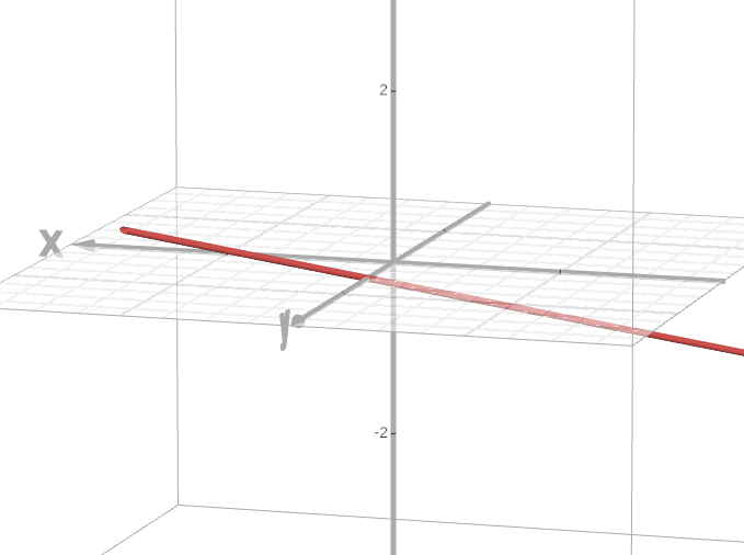
In 3-dimensional space, line equations are a bit more complicated than in 2d. While in 2 dimensions you might have a line with the equation x + 2y = 3, x + 2y = 3 in 3d space is a plane – an infinite flat surface. As it turns out, you can’t produce a line with just a single equation in x, y, and z: the system of equations x + y = 0; z = 0 is a line, but there’s no way to convert both of those constraints into a single equation. Dealing with systems of equation is clunky, so the preferred way to think of lines in 3d space is as a point plus t times a vector, where t is everything between -infinity and infinity. The representation of a 3d line is thus like so: r(t) = <0, 1, 0> + t * <2, 3, 0>, which in desmos 3d looks like this:
The vector equation form has many benefits over other methods of writing line equations, not least that you can very quickly determine a vector parallel to a line (it’s just the vector multiple of t!) and a plane perpendicular to it (we’ll get to that in a bit).
This sort of representation also means that it’s very easy to solve problems of the form “write an equation for a line passing through point p parallel to vector v”: the answer is just r(t) = p + tv!
You can also write the line as a system of equations in terms of t. This is as simple as reading off the vector values. For instance, the system of parametric equations of <6, 4, 1> + <2, 3, 5>t is x = 6 + 2t, y = 4 + 3t, z = 1 + 5t. With a bit of algebra, you can reduce this to two equations in x, y, and z.
Another common problem is finding a line that passes through two points. In this case, the operation is once again quite simple: given points p1, p2, the line that passes through both is r(t) = p1 + (p2 - p1)t.
Finding the nearest point v on a line in the form r(t) = p + ts to the point u is as simple as translating to the origin and projecting: v = p + (u - p) . t / (t . t) * t. Finding the distance can be done easily from there, and there’s even a simplified equation: ||(u - p) x v|| / ||v|| (shamelessly copied from the Thomas calculus textbook).
In this vector form, it’s actually slightly harder to find the point at which two lines intersect. As far as I can tell, the textbook doesn’t actually include this, but it’s a problem that’s come up in class and in the homework. My solution is to reduce both lines to a system of equations in s and t and solve it, following these steps:
-
Set up the initial equation. For instance, if we have two lines r(t) = <0, 0, 0> + <1, 1, 1>t and f(s) = <2, 2, 0> + <-1, -1, -2>s, the equation to solve is <0, 0, 0> + <1, 1, 1>t = <2, 2, 0> + <-1, -1, -2>s.
-
Simplify: <1, 1, 1>t + <1, 1, 2>s = <2, 2, 0>.
-
This can now be converted into an augmented matrix multiple of !
-
Row-reduce. If you haven’t taken linear algebra, this Georgia Tech open source textbook section is a good walkthrough of the process. Now we’ve this matrix:
-
Converting this back into a system of equations, we now have t = 4 and s = -2! Plugging these into the line equations yields the intersection point <4, 4, 4>
Note that there are exception cases. Oftentimes, lines will “miss” each other, and the equations will not have a solution. There is another case where the parallel vectors are scalar multiples of each other, meaning the lines themselves are parallel (it’s important to distinguish this from the miss case!); finally, it’s possible for the equations to have infinitely many solutions, in which case the lines are equal.
Planes
Like 3d lines, plane equations can get messy fast. Fortunately, there is a vector way!
Given a point p that the plane passes through and a perpendicular vector v describing its tilt,
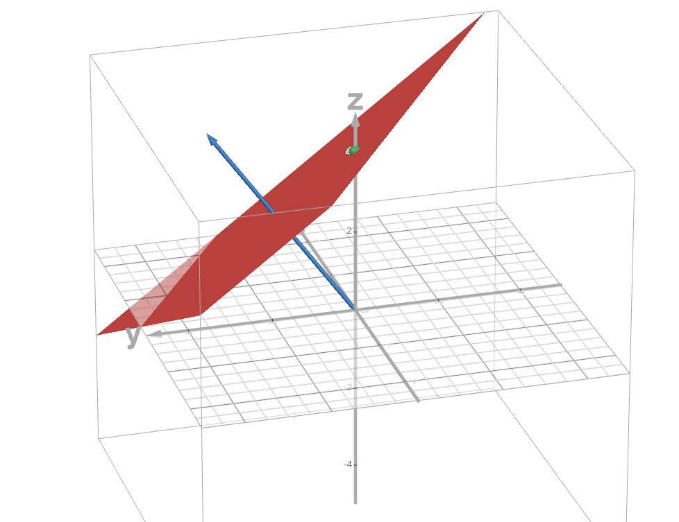
the equation for a plane is simply v . = v . p. For instance, a plane orthogonal to <2, 3, 4>
that passes through the point <0, 0, 4> is 2x + 3y + 4z = 16. Desmos 3d
is a good way to graphically inspect that this is indeed the correct plane equation:
This also means that any plane in the form Ax + By + Cz = D is orthogonal to . The vector equation for a line perpendicular to said plane would be r(t) = p + t – and if you have a line r(t) = p + vt, a plane perpendicular to it can be immediately found to be v . = 0!
Finding a plane that passes through several points is also fairly simple. To find, say, the plane through p1 = <2, 3, 1>, p2 = <0, 1, 5>, and p3 = <3, 3, 3>, we,
- Pick a starting point. This will go on the intersection side of the equation and be used as a basis for calculating the orthogonal vector. It doesn’t matter which one; for this, I’m using p1.
- Take the cross product (p2 - p1) x (p3 - p1). Because (p2 - p1) and (p3 - p1) are vectors perpendicular to the plane by definition, the cross product of them must be parallel to the plane. Note: there is an exception case; if the cross product is 0, the points are on the same line, and there are infinitely many planes passing through them all. In this case, (p2 - p1) = <-2, -2, 4>, (p3 - p1) = <1, 0, 2>, and <-2, -2, 4> x <1, 0, 2> = <4, -8, -2> (if you don’t know how I got this, I recommend reading the section on 3D Vectors).
- Construct the plane equation: <4, -8, -2> . = <4, -8, -2> . p1 => 4x - 8y - 2z = -18
Plane intersections are fairly easy to solve as systems of equations using some linear algebra, similar to the technique I described in the section on lines, but there’s a much less awful vector way to do it! We simply have to find a vector v parallel to the line of intersection of two planes and a point p common to them, and the line is r(t) = p + vt. For example, with the planes 3x - 6y - 2z = 15 and 2x + y - 2z = 5 (shamelessly copied from the Thomas textbook), the orthogonal vectors are <3, -6, -2> and <2, 1, -2>. The cross product of them gives us <14, 2, 15>, which is a vector parallel to the vectors parallel to the planes – the only possibilities for such a vector are parallel to the line of intersection between the planes.
Now we solve the intersection with the plane z=0, the result of which is a single point described by the system of equations: 3x - 6y = 15, 2x + y = 5. This yields a point <3, -1, 0>, so the line of intersection will be r(t) = <3, -1, 0> + <14, 2, 15>t. Not too difficult! Note that the third plane you intersect with doesn’t matter. z=0 is a simple, good choice, but you can intersect with any! The goal of intersecting with a third plane is just to isolate a single point on the line of intersection without actually solving for the line of intersection. You can use good ol’ algebra (or even row-reduction) to solve the problem, and probably faster, but then you have a gross system of equations instead of a nice vector-equation line – ultimately, doing things the vector way pays off in pain mitigation.
The distance from a point to a plane can be found by following this process:
- Pick a reference point on the plane: the intercepts are a good choice, because you can immediately zero two axes, so the x-intercept of a plane like 2x + 3y + 4z = 6 reduces to 2x = 6 -> x = 3, and thus the x-intercept is <3, 0, 0>.
- Offset your point by the reference point. For instance, if the point we’re measuring to is <5, 5, 5>, we’d subtract to get <2, 5, 5>.
- Project the offset point onto the plane’s normal vector. Because the normal vector here is clearly <2, 3, 4>, and the formula for projection is u * v / u . u * u, this is simply <2, 5, 5> . <2, 3, 4> / <2, 3, 4> . <2, 3, 4> * <2, 3, 4> = 39 / 29 * <2, 3, 4>.
- Take the magnitude of the projection. In this case, 39/29 * sqrt(29) = 39/sqrt(29) = ~7.24.
To instead find the nearest point on the plane, just add the reference point to the projection.
The angle between two planes is simply the angle between their normal vectors. See the section on 3d vectors for how to find that using the dot product and inverse trigonometry
Vector Functions
Vector functions are an extension of the idea of the vector equation of a line. Instead of strictly conforming to the r(t) = p + vt format, they are any function that outputs a vector. Generally this means each component will be a function of t. For instance, r(t) = is a vector-valued function.
A useful property of these is that, because component notation is interchangeable with vector notation, these can also be seen as functions comprised of the sum of multiples of i, j, and k, which are constants (see the section on vectors): r(t) = sin(t) * i + cos(t) * j + t^2 * k is identical to the previous r(t). This makes some operations very straightforward. For instance, taking the antiderivative of <1/t, t, 1> is the same as taking the antiderivative of 1/t * i + t * j + 1 * k – ln(t) * i + t^2/2 * j + t * k. This can then be reassembled into < ln(t), t^2, t>. In fact, it’s not even
necessary to expand the vector form: `int [ x(t), y(t), z(t) ] dt` is always `[int x(t) dt, int y(t) dt, int z(t) dt]`, so you can just integrate the components. The same goes for taking
the derivative: `d/dt [ x(t), y(t), z(t) ] = [d/dt x(t), d/dt y(t), d/dt z(t)]`. Limits of vector-valued functions are also taken the same way.
If the derivative of a scalar function is the instantaneous slope, the derivative of a vector function is the instantaneous direction. This is a surprisingly useful concept. For instance, the tangent line to a vector-valued function at s is r(t) = f(s) + f’(s).
Arc Length
The general formula for the length of the path described by a vector-valued function r(t) between a and b is
`int_a^b || r'(t) || dt` – the integral of the magnitude of the derivative of r(t). If r(t) is the sum of all of the infinitesimal instantaneous vectors in the curve preceding t (the integral of the derivative), then the length of r at t is the sum of all of the infinitesimal magnitudes preceding t. Rather than summing the instantaneous vectors of r(t), we’re summing the magnitudes of the instantaneous vectors of r(t).
For instance, the arc length of a simple line `l(t) = [0, 0, 0] + [3, 4, 0]t` between 0 and 10 can be found like so:
-
`l'(t) = `
-
`||l'(t)|| = sqrt(3^2 + 4^2 + 0^2) = 5`
-
`int 5dt = 5t`
-
`int_0^10 5dt = 50`
This can be quite complex to solve for some vector-valued functions. Fortunately, however, trigonometry makes some such problems very easy: for instance, the arc-length of
`r(t) = [2sin(t), 2cos(t), 1]` along `0 <= t <= 5`:
`r'(t) = [2cos(t), -2sin(t), 0]`
`||r'(t)|| = 2sqrt(cos^2(t) + sin^2(t) + 0)`, and because of hte pythagorean identity `cos^2(theta) + sin^2(theta) = 1`, `= 2`
`int 2dt = 2t`
`int_0^5 2dt = 10`
Simple!