Differential Equations Week 1

By Tyler Clarke in Calculus on 2025-5-17

Note: the next post in this series can be found here.

Hello, everyone! Break is over (for me, at least... the lucky buggers at KSU get another two weeks), and the first week of summer classes is almost over. As you probably can tell by the title, one of the classes I'm taking is differential equations - which means, of course, the entire Internet gets to hear about it. This course is looking like it will be quite daunting. To keep ahead, I'm going to be writing at least once weekly reviewing all of the material from the week and previewing at least some of the material for next week (Editor's note: this might be an overly lofty goal, considering how this week turned out).

The textbook I'm using is called "Differential Equations: An Introduction to Modern Methods", by James Brannen et al. You don't need it to follow this, but you really should get it anyways.

Some Review

Let's start with review. Much of this week was given to revisiting calc 2 concepts; I won't cover those in detail here, but if you're fuzzy on any of the following (nonexhaustive), you need to pay Salman Khan a visit:

• Integration by parts
• U-Substitution
• Trig integrals and derivatives (including reciprocals, squares, and antiderivatives!)
• Exponential and logarithmic integrals and derivatives

Differential Equations and the Variable Separable Method

We covered all of chapter 1 pretty quickly - it's only three simple introductory sections. The critical thing to understand is that there are some equations where the derivative of the independent variable depends on the independent variable. These are called differential equations. For instance, the famous Newton's law of cooling states that `frac {du} {dt} = -k(u - T)`, where `t` is time, `u` is the temperature of an object, `T` is the external temperature, and `k` is some arbitrary constant. This is called an ordinary differential equation because there is only one independent variable `t`. This equation is also first-order because the highest derivative of the dependent variable is the first one. If it had instead been `frac {du^2} {d^2 x}` (or `y''(x)`), this would be second-order, but that would be nonsensical.

Can you guess at a function that produces this behavior? If not, don't be alarmed - this is difficult to find with brute force. We'll cover a simple technique to solve this equation and find `u(t)` in a bit. Before we do that, we need to think about what a solution actually is. There are oftentimes many solutions and types of solution! For instance, in the case of Newton's law of cooling, there's a trivial solution when `u(t) = T`: if you substitute, you'll see this reduces to `0 = 0`. This is an equilibrium solution.

There is actually a very easy way to find a general solution. It relies on some truly awful algebra, but it works! This is called the variable separable method, and it relies on the differential equation being rewritten in the form `frac {dy} {dx} f(y) = g(x)`. In this form, you can multiply both sides by `dx` (note: this is technically very wrong, but it works!) to get `f(y) dy = g(x) dx`, and then integrate both sides. In the case of Newton's law of cooling, we can rewrite as `frac {du} {dt} frac {1} {u - T} = -k`. Multiplying both sides by `dt` gives us `frac {1} {u - T} du = -k dt`, and integrating gives us... `ln|u - T| + C_1 = -kt + C_2`. Because both `C`s are arbitrary constants, we can actually combine them: `ln|u - T| = -kt + C`. To isolate `u`, we need to raise `e` to both sides, to get `u - T = +- e^(-kt + C)`. This can be rewritten as `u - T = +- e^(-kt) e^C`, and because `+- e^C` is an arbitrary constant, we can actually munge that into just `C`. Some algebra gives us the final solution: `u(t) = Ce^(-kt) + T`. If you plug this into the equation, you'll see it's correct! We'll look into the variable separable method more in a bit.

Aside: Integral Curves and Initial Values

Equations that can be solved with the variable-separable method are the exception, rather than the rule; most differential equations are far too complicated. However, we can still find useful information (including equilibrium solutions) about them through graphical means. Because most differential equations will yield you `frac {dy} {dx}` with respect to `y` and `x` after some algebraic manipulation, you can use this knowledge to draw curves describing the behavior of the equation. As graphics are the antithesis of everything holy over here at Deadly Boring Math, I won't get too deep into this topic; consider visiting the textbook.

Knowing general solutions is nice and all, but what if we want to find a specific solution that encounters a given `(x, y)`? This category of problem is known as an initial value problem and is quite important to understand. Take, for instance, the cooling equation above: note that it doesn't actually tell us very much. It gets quite a bit more useful when we have some kind of constraint: for instance, we can say that, at time 0, the temperature is 45 degrees, and we're in an environment of 60 degrees. More formally: `u(0) = 45` and `T = 60`.

Let's substitute at `t = 0`: `45 = Ce^(-k * 0) + 60`. Obviously this is `45 = C + 60`, and then we can solve to find `C = -15`. Now we have a useful equation! `u(t) = -15e^(-kt) + 60` has no unknowns, so we can actually use it to predict the temperature at any given time `t`. Simple enough.

Autonomous Equations, Phase Lines, Direction Fields, Oh My!

A differential equation is considered to be autonomous if it can be written without the independent variable, in the form `frac {dy} {dt} = f(y)`. Autonomous equations are simpler to work with than non-autonomous, and there are a few operations that can be done on them to quickly discern useful properties of the equation. Critically, autonomous equations may have constant equilibrium solutions where the equation isn't changing - that is, when `frac {dy} {dt} = 0`. Equilibrium solutions have three classifications:

• Asymptotically Stable: Asymptotically stable equilibrium points are characterized by the fact that nearby solution curves will always converge on them. For instance, in the Newton's law of cooling example, the temperature will always approach equilibrium: every initial value you pick will produce a curve that converges on `T`. Thus, `T` is an asymptotically stable equilibrium point.
• Semi-Stable: Semi-stable equilibrium points are points where nearby curves will converge in one direction and diverge in the other.
• Unstable: The exact opposite of asymptotic stability; every nearby solution curve will diverge.

It's important to note that equilibrium point classifications are usually only local: it's possible to have multiple asymptotically stable points, for instance, where every solution curve converges to the nearer one.

Finding these equilibrium points is very easy: if we have a differential equation `frac {dy} {dx} = f(y)`, we can just set `frac {dy} {dx} = 0` and solve `f(y) = 0`. But what about classification? This is where we introduce a particularly useful concept (one so useful, in fact, that I'm willing to waive my desperate hatred of graphics for it): the phase line. Essentially, a phase line is a single axis representing every value of `y`. Every equilibrium point is graphed on it. To classify the equilibrium points, we pick several points between them and note the direction of the derivative with an arrow on the line. It might help to have an illustration:

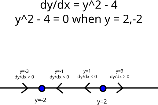You'll note that the equilibrium point at `y=2` is unstable because the derivative nearby is always pointing away from it; the equilbrium point at `y=-2` is asymptotically stable because the derivative nearby is always pointing towards it. The points `[-3, -1, 1, 3]` that I used for this are not picked by any magical rule; I just grabbed some numbers that were easy to evaluate `y^2 - 4` on and also close enough to both equilbrium points to get a good idea of the shape of the curve. Technically, I could have done without `-1` and `1` and just used `0`: we know the derivative doesn't change direction between two equilbrium points, because it would have to pass through 0, and there's an equilibrium point every time `frac {dy} {dx} 0`. Regardless, it doesn't matter which way you do it; adding an extra test point is rarely so much effort to be prohibitive.

It's useful to note that a phase line is really just a simplified special case of a solution curve graph: each equilibrium point corresponds to a straight line on the graph, and the convergence/divergence is made obvious by the curved lines. Generally, a phase line is much easier to construct and read than a solution graph; if your equation is autonomous and you need to visualize its equilibrium points, a phase line is much simpler than drawing a bunch of different solution curves. You get the same result but with much less headache!

`frac {dy} {dx}` across the `y`-axis is called the direction field because at each point it describes the direction the curve is pointing in. You can graphically represent this by drawing the `frac {dy} {dx}` vector at "every point" on the graph (practically speaking, you will have to pick an even spacing and draw at every interval). You'll note if you draw solution curves on this field that they line up with the direction field: this is for fairly obvious reasons.

One of the particularly useful properties of this geometric method is that you can use it to approximate non-constant solutions to a differential equation. Trace a curve through the field, following the direction vectors by "adding" each one to the tip of the curve, and repeat for a bunch of initial values: if the solution converges, you'll see the lines get closer and closer together until they look like a single line, and you can approximate the solution function by that.

Briefly: Refining the Variable Separable Method

Earlier, we did an example of solving a differential equation with the variable-separable method. It's a fairly straightforward technique and very powerful, albeit limited (many interesting differential equations cannot be separated). The core idea is that, if an equation can be written like `frac {dy} {dx} = p(x) q(y)`, you can do algebra to rewrite it as `frac {1} {q(y)} dy = p(x) dx` by pretending `dx` and `dy` are variables (they aren't, but it works). This equation can then be integrated on both sides, giving you a solution in the form `g(y) = h(x)`.

Let's do a slightly more complicated example. Helpfully provided by the textbook is `frac {dy} {dx} = frac {x^2} {1 - y^2}`. The goal of the variable-separable method is to find functions `q(y)` and `p(x)` where the equation can be rewritten as `frac {dy} {dx} = p(x) q(y)`; in this case, it's fairly clear that `p(x) = x^2` and `q(y) = frac {1} {1 - y^2}`. Inserting them in the form shown above gives us `frac {1} {frac {1} {1 - y^2}} dy = x^2 dx`, or `(1 - y^2) dy = x^2 dx`. Integrating both sides gives us `int (1 - y^2) dy = int x^2 dx => y - frac {y^3} {3} = frac {x^3} {3} + C`, which simplifies to `y^3 = 3y - x^3 + C`, or `y = root(3)(3y - x^3 + C)`.

Note: in many cases, it is not possible (or is very hard) to isolate `y` after solving the differential equation. In these cases, you have what is known as an implicit solution in the form `f(x, y) = g(x, y)`, as opposed to an explicit solution in the form `y = f(x)`. It's critical to remember that implicit solutions are sometimes all you need!

Method of Integrating Factors

There are quite a few different ways to find the (analytiC) solution to a differential equation. We've already covered the simplest one (the variable separable method); unfortunately, it is quite limited. We need a more powerful approach. A method that can handle any differential equation in the form `frac {dy} {dx} + p(x}y = g(x)` (known as a first order linear differential equation) is the method of integrating factors.

The derivation is not too hard, but I won't include it here for brevity; I highly recommend reading the textbook (section 2.2) to understand why this works. The step-by-step solution is thus:

1. Convert the equation to the linear form `frac {dy} {dx} + p(x)y = g(x)`. If you can't do this, the rest won't work.
2. Find the integrating factor `mu`. This is always `mu = e^{int p(x) dx}`, for truly fascinating reasons. Read the book!
3. Rewrite as `frac {d} {dx} (mu y) = mu g(x)`. This is the most magical part.
4. Integrate, to get `mu y = int mu g(x) dt`.
5. Solve!

This is quite difficult, so let's do an example with the equation `x frac {dy} {dx} + 2y = 4x^2`. First off, we need to rewrite in linear form, by dividing the whole thing by `x`: `frac {dy} {dx} + frac {2y} {x} = 4x` (this requires that `x != 0`). It's clear in this form that `p(x) = frac {2} {x}` and `g(x) = 4x`. `mu = e^{int frac {2} {x} dx} = Ce^{2ln|x|}` (not sure where `C` came from? It's the same trick as in the variable-separable method). Here lies a dangerous pitfall: if we leave `mu` in this form, the next few steps will be extremely difficult. Fortunately, logarithms are on our side! We know that `e^{ln|x|} = |x|`, so `mu = Cx^2`. Much nicer. We continue with `Cx^2y = int 4Cx^3 dx`, which evaluates to `Cx^2y = Cx^4 + C_2`. Finally, divide both sides by our first arbitrary constant and recombine constants, to get `x^2y = x^4 + C`. Not too bad!

It's highly recommended to simply memorize the method of integrating factors, rather than try to memorize the proof.

A Brief Splash of Preview

Judging by the worksheets, next week will be covering section 2.3 and 2.4. Let's do a problem from each (pulled from the textbook).

First up is constructing a mathematical model of a dilution tank (we actually did a similar one in lecture). The textbook uses loathesome imperial units, so I've made up some reasonable metric ones for consistency. We're given a tank containing a magic stirring device that very quickly equalizes the concentration of salt in water in real time. The tank starts with `Q_0` grams of salt dissolved in 100 liters of water. Water containing 10 grams of salt per liter is flowing in at `r` liters per second; fully-mixed water is also flowing out at the same speed. We need to find the amount of salt in the tank at any given time.

Let's dive right in by finding a differential equation describing the amount of salt in the tank. The flow rate of salt is the flow rate of the incoming water times the concentration: this gives us `s_"incoming" = 10r` grams per second. Trouble strikes when we consider outgoing salt: the amount of salt leaving is related to the amount of salt in the tank, which is the outflow rate times the current concentration. Because the tank is holding a constant 100 liters, concentration is always `frac s {100}`, so `s_"outgoing" = frac {sr} {100}`. Because we know both of the components, we know the total change in salt concentration `frac {ds} {dt} = 10r - frac {sr} {100}`.

This is actually a linear differential equation! If we rewrite, we get `frac {ds} {dt} + frac {sr} {100} = 10r`. This lines up perfectly with the form `frac {ds} {dt} + p(t)s = q(t)`, where `p(t) = frac r { 100 }` and `q(t) = 10r`.

The integrating factor here, then, is `mu = e^{int p(t) dt}`, which is just `Ce^{frac {rt} {100}}`. Inserting into our convenient equation gives us `Ce^{frac {rt} {100}}s = int 10r Ce^{frac {rt} {100}} dt`. Integrating that is actually surprisingly easy: we get `Ce^{frac {rt} {100}}s = 10r frac {100} {r} Ce^{frac {rt} {100}} + C_2`, which simplifies to `e^{frac {rt} {100}}s = 1000 e^{frac {rt} {100}} + C` by merging constants and doing some elimination. Finally, we can transform this into `s = 1000 + Ce^{- frac {rt} {100}}` by dividing by the integrating factor. This is the solution!

Section 2.4 introduces an interesting way of determining if a linear differential equation has a solution at all: check the domain of the components. If both `p(t)` and `q(t)` are defined along some interval `I` that contains the initial point, then there is a solution for every `t` in `I`, which fully satisfies the initial condition.

Let's do an example. We're asked to find an interval in which the following initial-value problem has a unique solution: `y' + frac 2 t y = 4t`, where `y(1) = 2`. We can read off that `p(t) = frac 2 t` and `q(t) = 4t`: `q(t)` is defined for every possible value of `t`, and `p(t)` is defined for `-oo < t < 0, 0 < t < oo`. The initial value `t_0 = 1`, which satisfies `g(t)` implicitly and satisfies the second range for `p(t)`, so our IVP has a solution in the range `0 < t < oo`. Easy enough! There's quite a lot more to think about with this, but I'll leave it off here until next week.

Final Notes

This ran quite a lot longer than I was expecting - it's now second only to my multivariable exam 1 review. I'll try to keep it more brief next week.

My Deadly Boring Math posts are not meant to be treated as complete study guides. The problems I work here are usually a little simpler than the ones we actually cover in class, per experience in multi; if this is all you use to prepare, you will not pass. My goal here is to provide interesting, somewhat-plain-English review material that forces me to think seriously about the topics (it may be a weird way to study, but it works) and helps other people pinpoint what they need to practice.

I am not an academic professional or expert in any of the things covered here. This means I'm not always right, and I don't always explain complex concepts in a good way. If you noticed something wrong, missing, or badly explained, please contact me!

If you're a professor or TA reading this, thanks for putting some time into reading my lil blog! I would love to hear any feedback you have on how I presented the material here; the best way to reach me is through my gatech email address, but my public-facing plupy44@gmail.com also works.

For my fellow students in Differential Equations at Georgia Tech Summer '25- there is a quiz next week (Thursday, May 22nd). Make sure to do all the applicable homework sections and worksheets and solve some of the extra problems! If you have notes of your own that you'd like to publish here, or have questions/comments/concerns, contact me at the above email address.

One final point of order: I intend to show up to every quiz and test in this class wearing a hat covered in balloons. I am completely serious. If this post was helpful to you, consider wearing one too! I can't guarantee wearing a balloon hat will make the quiz go better, but it will certainly go more hilariously. Maybe it'll become a trend.

Tune in next week for the thrilling conclusion!