Math Gun pt. 1

By Tyler Clarke in Physics on 2025-5-2

Hello once more, gentle readers! I hope everyone's having a decent break and won't be suffering from boredom this summer. Today we're covering a much-awaited topic: railguns! When I first learned about magnetism in physics, the very first thing I thought was - "wait, I can make a math gun". Railguns have always fascinated me, and now that I actually understand the fundamental principles behind them, naturally I want to build one.

I'm gonna do this in three sections. The first one (this one) will cover building the initial mathematical model: an equation relating all the properties of a parametric math gun (is that an official term? no. no it is not), including properties of the circuit (like the capacitor grid). The second section will cover building a computational model to visualize (and verify) the results - and the last section will involve actually building the railgun with the kind folks over at Scrappy's Garage, who unlike me have the equipment to manufacture a railgun.

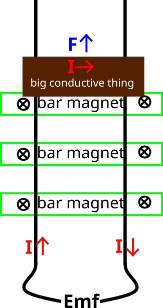The basic design of a railgun relies on a property of circuits and magnetics: `F = IL times B` - the force on a current segment is equal to the length of the segment, times the magnitude of the current, times the direction of the current, cross with the magnetic field around it. Railguns, then, work by running a current in the `hat x` direction through a conductive object, and using permanent magnets to produce a sustained magnetic field across that object in the `hat z` direction. This leads to a net force in the `hat x times hat z = hat y` direction. The easiest way to generate that current is with a pair of powered rails.

The attractive thing about railguns is that they can produce a powerful shot, even in a fairly low-power system. A small drone battery might produce a 5A max current, and you can pretty easily get magnets that will produce a field in the ballpark of 1T. Because the directions are all perpendicular, we can multiply the magnitudes directly on the cross product; a fairly small (5cm) rail weighing 10 grams in that field under these conditions will experience several gravities of acceleration (25 meters per second squared). Consider the highly idealized case of an object experiencing this acceleration across a 50cm rail: `frac 25 2 t^2 = 0.5 -> t = sqrt(frac 1 25)`, working out to an exit velocity of `v = 25t = frac 25 5 = 5` meters per second. That's pretty fast for a launch from a fairly small, weak assembly! However, this is an oversimplified model. To get anything like accuracy, we need to consider air friction, mechanical friction, and self-induction. Let's do air friction first.

The general formula for drag is `F_d = frac 1 2 v^2 p C_d A`: the drag force is one half of the velocity squared, times the density of the fluid, times the drag coefficient, times the cross sectional area. This obviously isn't a perfect model, but I don't want to build a CFD simulation, so it'll have to work. If we assume the object we're launching is a 1cm diameter ball bearing (weighing ~4 grams - it's shockingly hard to find this size, but McMaster comes in clutch as always), we're looking at a circular cross-section of `pi 0.005^2` regardless of orientation. The drag coefficient of a sphere is `0.47`, and the density of atmosphere at sea level is `1.225` kilograms per meter cubed, so we're looking at a drag force of `F_d = frac {0.47 * 1.225} 2 pi 0.005^2 v^2`, or `~9*10^{-5} v^2`. This means the formal equation for force on our marble (normalized to the y direction only) is now `F = 0.01IB - 9*10^{-5} v^2`. Acceleration is simply that divided by mass. Because velocity is the integral of acceleration, and we're starting from 0, we have this little formula: `v = frac 1 0.004 int_0^t 0.01IB - 9*10^{-5} v^2 dt`. This is a very difficult integral to calculate; let's table it for now. Until we reach fairly high velocities, we don't have to worry much about this.

Let's now worry about induction. As the marble moves through the magnetic field, it induces a current in the rails opposing the one running through it - this is Faraday's and Lenz' law. This induced electromotive force is equal to `- frac {d phi} {dt}`, where `phi` is the magnetic flux through a given loop. Magnetic flux is simply the surface integral of magnetic field over the inside of the loop - in this case with uniform `B`, it's just the magnetic field times the area. Taking `L` to be the distance between wires, flux is thus `B L y`, where `y` is the height of the loop. We don't have to know `y` rigorously; we just need to know the change in `y`, which is `frac {dy} {dt} = v`. Because the other terms are constant, this means `- frac {d phi} {dt} = -BLv`. That's the induced voltage! This means our voltage at any given time is `V = Emf - BLv`. That's very easy to plug into our above formula: Ohm's law gives us `I = frac V R`, so the full equation is now `v = frac 1 0.004 int_0^t 0.01B frac {Emf - BLv} {R} - 9*10^{-5} v^2 dt`.

This is an extremely hard integral to find - even Wolfram|Alpha has no idea. We'll have to build a computational model.

There's one more thing to do before wrapping this up: we need to consider capacitors. For those not in the know, a capacitor is essentially a short-term battery that charges and discharges comparatively quickly. The attractive thing about capacitors in this situation is that they can be used to turn a battery's continuous low voltage into a brief push of very high voltage.

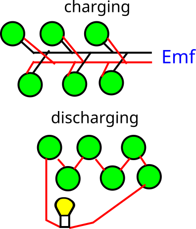
You can see in the graphic to the right an example of a voltage source charging a bunch of capacitors in series: I won't go into the nitty-gritty details of how this works on a micro level (although it is quite fascinating). This will take a long time: note that it is in parallel, so the voltage across each capacitor will be charged up to `Emf`. When discharging, the capacitors are switched into series: remember the Loop Rule of a circuit - the voltages will add, meaning the total voltage through the bulb is `5 Emf`. The tradeoff is that, of course, we won't get a sustained voltage this way: we'll have to spend 5x as much time charging as discharging. For a system like a railgun, this is quite ideal: we have a capacitor grid that charges from a battery until we fire a shot, then discharges into the rails until the shot finishes (this would have to be managed by a microcontroller switching solid state relays - we'd use a hall effect sensor to determine when no current is running through the rails, meaning the marble has left the track). We can tune the duration of capacitor discharge with a resistor.

Tuning properties of the capacitor grid and resistor(s?) will likely require brute-force sampling with a computational model; to do that we'll need to have some formulas to compute. Given that the base resistance of the railgun is `R`, and the added resistor is in series with the railgun, our total resistance is `R + R_"add"`. Let's also assume we're using `N` capacitors with capacitance `C`, so our final series voltage is `V = N "Emf"`. Capacitors charge by an exponential function `Q = C"Emf"(1 - e^{- frac t {RC}})`, and `V = frac Q C`, so our capacitor voltage in terms of time is `V(t) = "Emf"(1 - e^{- frac t {RC}})`. This will clearly never reach `"Emf"`, but will quickly approach it - if we want to know the time `t` at which we'll have reached a voltage `V_"targ"`, we solve `V_"targ" = "Emf"(1 - e^{- frac t {RC}})` to get `t = -RC ln(1 - frac {V_"targ"} {"Emf"})`. `1 - frac {V_"targ"} {"Emf"}` is very convenient for our purposes: for instance, if we want to get within 20%, it's just `ln(0.2)`. Assuming we're using larger capacitors on the order of millifarads, and the charging circuit has in the ballpark of 0.01 ohms of initial resistance (this is reasonable, although maybe a bit conservative based on copper wire numbers), then `RC` is on the order of `0.00001`. This gives us 16 microseconds to an 80% charge, 23 micros to 90%, and about 30 microseconds to 95%. Note that this is true for any voltages - a dinky 3.3v battery array and a chonky 120v wall socket supply will both charge our lil' 1mf capacitor to 95% in 30 microseconds (although the wall socket is significantly more likely to blow it up - don't try this at home). Because we're charging in parallel, we logically just multiply by `N` to get the total time to charge the entire grid.

There is a lot more complexity with capacitors (and price... jeez, $50 for a single capacitor), but it's not useful to theorize about the capacitor grid much more without some concrete simulation and bench test results. See you next time with a computational model!